Data Acquisition
Stuart Hertzog
May 16, 2018
Data acquisition tools are built into R, which makes it extremely easy to access large pools of publicly-available statistical data pools that have been assembled by governments, research centres, corporations, business associations, non-profit organisations, and individuals.
Data can be harvested from:
- Plain text and delimited files (
.txt,.csv,.tsv) - Microsoft Word and Excel files (
.doc,.docx,.xls,.xlsx) - Data contained within databases (SQLite, MySQL, Microsoft Access)
- Data in statistical software (SAS, SPSS, NCSS, Octave)
The data sources can be located:
- in
RandR packages - on your computer storage
- on a local or linked network, or
- anywhere on the global Internet
Built-In R Datasets
An R installation includes many built-in datasets. These are contained in the package datasets and are available at all times. They can be listed with the command:
Specific datasets can be loaded using the same data() function and its structure inspected using head():
Datasets In Packages
Many packages also contain their own datasets. A package must be installed and loaded before its dataset is available. You can see a comprehensive listing of the datasets included in all installed packages with the command:
Packages will be listed in alphabetical order followed by the datasets they contain. You will be surprised to see how many datasets are available for your use! Due to changes in dataset organisation in recent R versions, you may see in Console:
Warning messages:
1: In data(package = .packages(all.available = TRUE)) :
  datasets have been moved from package 'base' to package 'datasets'
2: In data(package = .packages(all.available = TRUE)) :
  datasets have been moved from package 'stats' to package 'datasets'
To import and inspect a dataset contained in a package:
Importing Delimited Data
Delimiter-separated data files are plain text files in which the data is arranged in rows, each row containing data items separated by a delimiter and the row ended by a <NEWLINE>. The first row of data is usually the column headings.
These are the most basic type of dataset as being plain text, they are cross-platform and can be opened by any text editor. Most database and spreadsheet programs are able to read or save data in a delimited format.
The most common data delimiters are:
- Comma-Separated Values (CSV –
.csvfile extension) - Tab-Separated Values (TSV –
.tsvfile extension) - Any other ASCII character (colon
:, pipe|, etc.) - Designated ASCII Control characters.
If the data items consist of multiple words or characters separated by punctuation or spaces, each data item must be contained within pairs of single '<ITEM>' or double "<ITEM>" quotes.
Using read.table
read.table is part of R’s built-in utils package. It’s the easiest way to import delimited data files, and results in a data.frame.
Here are the first six lines of a .csv file containing data from a Fitbit tracker. It is called fitbit-activity.csv and is located in the docs directory of this project:
theFile <- "docs/fitbit-activity.csv"
fitbit <- read.table(file=theFile, header=TRUE, sep=",")
head(fitbit)
read.table has three arguments:
- The path and filename or URL of the data file;
- Path can be absolute or relative to the current working directory;
- Whether the first line contains the column header labels;
- set to TRUE if and only if the first row contains one fewer fields than the number of columns; and
- The separator between data items.
- If not set, the default is
""white space, meaning one or more spaces, tabs, newlines or carriage returns. This can be set to\t() or ;(semicolon) as appropriate.
- If not set, the default is
Documentation of read.table can be viewed with:
Two important arguments are:
as.is– the default behavior ofread.table, converts character variables to factors, whilestringsAsFactors–TRUEorFALSEcan be used to prevent this, althoughas.isandcolClasses, which sets the data type for each column, will override it (see the documentation).
Pre-set Wrappers
read.table has wrappers pre-set for different file delimiters:
| Function | separator | decimal |
|---|---|---|
| read.table | empty | period |
| read.csv | comma | period |
| read.csv2 | / | comma |
| read.delim | \t | period |
| read.delim2 | \t | tab |
If you know the delimiter, using one of these is the easiest way to import those files.
read.table is slow to read large files into memory. Two other packages provide function that are faster and better in that they do not automatically convert character data to factors:
read.delimfrom thereadrpackage by Hadley Wickham, andfreadfrom thedata.tablepackage by Matt Dowle.
Using readr
The readr package handles many kinds of delimited text files:
read_csv()– comma separated (CSV) filesread_tsv()– tab separated filesread_delim()– general delimited filesread_fwf()– fixed width filesread_table()– tabular files where colums are separated by white-space.read_log()– web log files
readr is much faster than read.table, and it also removes the need to set stringsAsFactors to FALSE since that argument does not exist in readr, which leaves strings “as-is” by default. It also shows a helpful progress bar with very large files.
Let’s open the same fitbit-activity.csv file with the read.delim() function:
## Parsed with column specification:
## cols(
##   Date = col_character(),
##   TotalSteps = col_integer(),
##   TotalFloorsClimbed = col_integer(),
##   TotalCaloriesBurned = col_integer(),
##   TotalElevationGained = col_double(),
##   TotalElevationGainedUnit = col_character(),
##   TotalDistanceCovered = col_double(),
##   TotalDistanceCoveredUnit = col_character(),
##   SedentaryMinutes = col_integer(),
##   LightlyActiveMinutes = col_integer(),
##   FairlyActiveMinutes = col_integer(),
##   VeryActiveMinutes = col_integer()
## )
readr returns data as a tibble, a modern re-imagining of the data.frame.
A tibble displays the file’s metadata under each column head, such as the number of rows and columns and the data types of each column. The tibble is also intelligently adjusted to fit the screen.
We can see this by examining the first few rows with head():
readr also has special cases for different delimiters:
read_csv()– for commas (,)read_csv2()– semicolons (;)read_tsv()– tabs (\t)
More information on read.delim() can be found in the readr documentation:
Using fread
The fread() function from the data.table package also will also read large data files faster than read.table, with the stringsAsFactors argument set to FALSE by default.
(You may have to install this package by entering install.packages("data.table") in the Console pane).
library(data.table)
theFile <- "docs/fitbit-activity.csv"
fitbit <- fread(theFile, sep = ",", header = TRUE)
fitbit
fread produces a data.table, an extension of data.frame. You can see the documentation for this data structure by entering ?data.frame in the Console.
Using RStudio
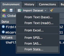
RStudio has tools to import delimited data. These are accessible from the Import Dataset tab of the Environment pane.
The two tools for plain-text delimited files are:- From Text (base)… – using base R
-
From Text (readr)… – using
readr
Instructions on their use can be found here.
Importing Excel Data
Prior to the more widespread use of R for Data Science, data was compiled in spreadsheets, mostly in Microsoft Excel, intially released in 1987.
Excel has a very different data structure from that required by R, and until recently it was difficult to bring Excel data sets into R.
The readxl package by Hadley Wickham has changed this, making it easy to import data from a single Excel sheet into an R project. However, the file must be present on the local computer.
fitbit-export.xlsx, a record of daily activities and nocturnal sleep, is available in the docs/ directory of this project.
It can be brought into R after you have loaded the read_excel package by entering install.packages("read-excel") in the Console pane.
Note: Depending on your version of R, you may have to install the development version by entering devtools::install_github("tidyverse/readxl") in the Console pane.
To do this you will first need to install the devtools package, obtained with install.packages("devtools").
Using `readxl
First check which sheets are in the Excel file:
## [1] "Activity data" "Sleep data"read_excel reads one sheet, by default the first, and displays the result as a tibble:
There are two ways of reading the second and subsequent sheets:
- by sheet number
- by sheet name
Unlike the previous two packages, read_excel cannot grab files from the Internet. They must be downloaded first either by copying and pasting the raw data from a Web browser, or by downloading them using the download.file package.
The command for download.file is entered in the Console pane, in the format:
download.file(url, destfile, method, quiet = FALSE, mode = "w",
              cacheOK = TRUE,
              extra = getOption("download.file.extra"), …)
You can also read the documentation for this package in the Viewer pane of RStudio by entering ?download.file in the Console pane.
RStudio’s built-in Import Tools also can handle Excel data (see above)
Importing JSON
JavaScript Object Notation (JSON) is an open-standard file format that uses human-readable text to transmit data objects consisting of attribute–value pairs and array data types. It is widely used for asynchronous browser–server communication – Wikipedia
Although JSON files are plain text, they can carry more complex data than delimited text or Excel files. They can contain nested data as arrays, even arrays within arrays, and because they are plain text they can be used for browser/server data communication.
Here’s an example of a JSON file:
{
    "glossary": {
        "title": "example glossary",
        "GlossDiv": {
            "title": "S",
            "GlossList": {
                "GlossEntry": {
                    "ID": "SGML",
                    "SortAs": "SGML",
                    "GlossTerm": "Standard Generalized Markup Language",
                    "Acronym": "SGML",
                    "Abbrev": "ISO 8879:1986",
                    "GlossDef": {
                        "para": "A meta-markup language, used to create markup languages such as DocBook.",
                        "GlossSeeAlso": ["GML", "XML"]
                    },
                    "GlossSee": "markup"
                }
            }
        }
    }
}
A JSON file can be found at docs/tidepool.json in this project. It is a selection from a much larger (1.9GB) JSON file downloaded from the Tidepool diabetic data repository, a user-contributed data repository available for diabetes-related Data Science research. This data was originally uploaded to Tidepool from an Abbott Freestyle Libre flash glucose monitoring (FGM) meter.
Using jsonlite
The R package jsonlite was developed specifically to bring JSON data into R. It can be installed by entering install.library("jsonlite") in the Console pane, after which the library can be loaded and used:
To just examine the structure:
Getting Started With jsonlite is available online and in its vignette, which you can view in RStudio by entering ??jsonlite in the Console pane and clicking jsonlite::json-aaquickstart.
A detailed example of working with JSON files can be found here.
Data In R Binary Files
RDS files are binary files that represent R objects of any kind. They use the
.rdataextension; can store a single object or multiple objects; and can be passed among Windows, Mac and Linux computers for use in those operating systems.
Save All Objects
To explore this, create an RDS file from the fitbit dataframe in memory:
To show the use of the RDS file, remove fitbit from memory:
If you test for it presence with head(), you will see the error message:
Error in head(fitbit) : object 'fitbit' not foundRestore it from the fitbit.rdata file:
Save One Object
The load() function stores all the objects in an RDS file, including their names. The saveRDS() function saves just one object to a binary RDS file, but without a name, so when loading it with readRDS it must be assigned to an object.
Create a vector:
## [1] 1 2 3 4 5Save it to an RDS file:
Read it to another object:
## [1] 1 2 3 4 5Check they are identical:
## [1] TRUESave Entire Workspace
The function save(image) will save all objects currently in your workspace. You must use the .rdata file extension for this:
The objects can be loaded into a workspace with load() function. These will overwrite existing workspace objects, so you may want to check what they are with:
##  [1] "activity"    "diamonds"    "fitbit"      "mtcars"      "MyVector"
##  [6] "sleepname"   "sleepnumber" "theFile"     "tidepool"    "USArrests"
## [11] "YourVector"
You can clear all workspace objects with:
You’ll see them disappear from the Environment pane. They can be loaded back with:
Save Session
RStudio saves the current workspace in its <projectname>.RData file. When you quit an RStudio session, you will be asked whether you wish to save the Session. This will save both the current variables and functions, so you will be able to pick up where you left off in a subsequent RStudio session.
However, some advise not to do that.
If you change the Working Directory you will need to load() the workspace to sync it to the new working directory.
RStudio enables workspace management from the Session menu:
- Load Workspace…
- Save Workspace As…
- Clear Workspace… and
- Quit Session…
Data From Databases
Most of the available data is held in databases, including Microsoft Access, Microsoft SQL Server, MySQL, or PostgreSQL.
To access a database, an ODBC connection is needed. Open Database Connectivity (ODBC) is a standard application programming interface (API) for accessing database management systems (DBMS). It is independent of operating systems and can be ported to all platforms.
RPostgreSQL, RMySQL, ROracle, and RJDBC are database-specific R packages, but if the database you wish to query doesn’t have a specifc package, the generic RODBC package is available. (Complete documentation here (PDF))
To help with database connection, the DBI package can be used.
DataCamp has two comprehensive tutorials on database connectivity: Part1 and Part 2.
Using RSQLite
First install the RSQLite and DBI packages by entering install.packages("RSQLite, DBI") in the Console pane.
Now load RSQLite and DBI packages to access the downloaded database:
To connect, first specify the driver using the dbDriver function :
## [1] "SQLiteDriver"
## attr(,"package")
## [1] "RSQLite"
Now connect to the tidepool database using the dbConnect function:
## [1] "SQLiteConnection"
## attr(,"package")
## [1] "RSQLite"
List the tables in fitbitactivity database:
## [1] "fitbitactivity"List the fields in the fitbitactivity table:
## [1] "Date,TotalSteps,TotalFloorsClimbed,TotalCaloriesBurned,TotalElevationGained,TotalElevationGainedUnit,TotalDistanceCovered,TotalDistanceCoveredUnit,SedentaryMinutes,LightlyActiveMinutes,FairlyActiveMinutes,VeryActiveMinutes"Now you are connected to the downloaded database and know its fields, you can make any SQL query and use dbGetQuery to return the result as a data.frame. (For more on SQL queries, W3Schools has an SQL Tutorial.)
It’s a good idea to set stringsAsFactors to FALSE to cut processing time and preserve Character data as character – dbGetQuery has this argument.
You should close the ODBC connection using dbDisconnect, although it will close automatically when the R session closes or you open another connection.
Data from Web Sites
In HTML Tables
Web pages often include data enclosed in an HTML Table. This data can be captured and examined using the XML package.
The XML package can parse and generate all types of XML data. XHTML and HTML5 now widely used on the Web are XML-compliant versions of HTML.
Using XML
First install the package by entering install.packages("XML") in the Console panel, followed by a RETURN.
Use the page URL to access the data inside an HTML table contained on a Web page. If the page has more than one table, set which (see example below) to the order number of the table you want to acquire.
NOTE: The readXMLTable function will NOT work with https:// URLs. You must use the http:// format of a URL only. You can also examine a file on your computer by giving the file path without the URL.
library(XML)
theURL <- "http://r.stuzog.com/docs/fitbit-activity-table.html"
fitbtable <- readHTMLTable(theURL, which=1,
             header=TRUE, stringsAsFactors=FALSE)
fitbtable
In Other HTML Elements
Not all useful data is contained in HTML tables. Some may be in ordered or unordered lists, <span>s, or other HTML elements. How to identfy and extract it?
Using rvest
The rvest package was designed by Hadley Wickham to do just this. Install it by entering install.packages("rvest") in the Console pane.
Let’s use the example tutorial by Hadley Wickham:
## Loading required package: xml2##
## Attaching package: 'rvest'## The following object is masked from 'package:XML':
##
## xml## The following object is masked from 'package:readr':
##
## guess_encoding## {xml_document}
## <html xmlns:og="http://ogp.me/ns#" xmlns:fb="http://www.facebook.com/2008/fbml">
## [1] <head>\n<meta http-equiv="Content-Type" content="text/html; charset= ...
## [2] <body id="styleguide-v2" class="fixed">\n <img height="1" ...That doesn’t tell us too much about the content of the page, so we need to have the Lego movie page open in our Web browser.
Using selectorgadget
To find the structure, Wickham recommends the open-source tool selectorgadget. You can read his documentation of this useful Web utility by entering vignette("selectorgadget") in the Console pane.
He uses html_node() to find the first node that matches that selector, extract its contents with html_text(), and convert it to numeric with as.numeric():
## [1] 7.8He suggests a similar process to extract the cast, using html_nodes() to find all nodes that match the selector, converting it to text with html_text():
##  [1] "Will Arnett"     "Elizabeth Banks" "Craig Berry"
##  [4] "Alison Brie"     "David Burrows"   "Anthony Daniels"
##  [7] "Charlie Day"     "Amanda Farinos"  "Keith Ferguson"
## [10] "Will Ferrell"    "Will Forte"      "Dave Franco"
## [13] "Morgan Freeman"  "Todd Hansen"     "Jonah Hill"
Web scraping is an art. Here’s a more advanced tutorial that may help.
From Other Software
R is not the only statistical software. Proprietary commercial and open-source formats pre-exist the popularity of R, provided by SAS, SPSS, and Octave, among others.
Using foreign
The foreign package enables reading data into R, returning it as a data.frame — if it succeeds, which often it does not. It includes the following functions for acquiring data from other statistical software:
| Function | Format |
|---|---|
read.spss |
SPSS |
read.dta |
Stata |
read.ssd |
SAS |
read.octave |
Octave |
read.mtp |
Minitab |
read.systat |
Systat |
Note: read.ssd normally requires a valid SAS license, but this can be circumvented by using Microsoft Machine Learning Server, which has the RxSasData() function in its RevoScaleR package.